Chapter 7 Approximations of trial solutions, weight functions and guass quadrature for multidimensional problems

Improve the solution of the finite element soulutions: 1) Element size \(h\rightarrow0\) , 2) Higher order approximation polynominal

Isoparametric element ---> treat curved boundaries and able to represent a linear field exactly

Triangular elements

Three node triangular elements

Three nodes lienar element

Six nodes quadratic element

Ten nodes cubic element

P 160

For quartic or higher order element are seldom developed from simple polynominal expansions.

In addition, these higher order elements will result in not well conditioned discrete system equations

Other high-order elements like spectral elements developed legendre polynominals will not degrade the conditioning as much

Triangular coordinates

\(\xi_I=\frac{A_I}{A}\), which is equal to the shape function of linear triangular elements

P175 The more distorted the element, the less its accuracy.

---

Quadrilateral elements

The construction of shape function \(\pmb{N}^e\) \(\Downarrow\)

• tensor product method ---> Lagrange elements

Taking products of lower dimensional shape functions and exploiting the Kronecker delta property

• Serendipity

Tensor product of carefully selected functions to satisfy the Kronecker delta property

Four node rectangular elements

Tensor product method

\(N^e_{K}(x,y)=N^e_{[I,J]}(x,y)=N^e_{I}(x)N^e_{J}(y)\) for \(I=1,2\) and \(J=1,2\)

Four node quadrilateral elements

Isoparametric element: The physical coordinates are mapped by the same shape functions as those for approximation

\(x(\xi,\eta)=\pmb{N}^{4Q}\pmb{x}^e\), \(y(\xi,\eta)=\pmb{N}^{4Q}\pmb{y}^e\)

\(\theta(\xi,\eta)=\pmb{N}^{4Q}\pmb{d}^e\)

Mapping from the parent to the physical coodrinates system

Derivatives of isoparametric shape functions

\(\pmb{\nabla}\theta=\pmb{B}^e\pmb{d}^e\) where \(\pmb{\nabla}=[\frac{\partial}{\partial x},\frac{\partial}{\partial y}]^T\)

Use the chain rule

$\begin{bmatrix} \frac{\partial N_I^{4Q}}{\partial \xi}\ \frac{\partial N_I^{4Q}}{\partial \eta} \end{bmatrix}= \begin{bmatrix} \frac{\partial x}{\partial \xi} & \frac{\partial y}{\partial \xi}\ \frac{\partial x}{\partial \eta} & \frac{\partial y}{\partial \eta} \end{bmatrix} \begin{bmatrix} \frac{\partial N_I^{4Q}}{\partial x}\ \frac{\partial N_I^{4Q}}{\partial y} \end{bmatrix} $

\(\pmb{G}\pmb{N}^{4Q}_{I}=\pmb{J}^e\pmb{\nabla}\pmb{N}^{4Q}_{I}\)

\(\pmb{B}^e=\pmb{\nabla}\pmb{N}^{4Q}_{I}=(\pmb{J}^e)^{-1}\pmb{G}\pmb{N}^{4Q}_{I}\)

where \(\pmb{G}=[\frac{\partial}{\partial \xi},\frac{\partial}{\partial \eta}]^T\), \(\pmb{J}^e=\begin{bmatrix} \frac{\partial x}{\partial \xi} & \frac{\partial y}{\partial \xi}\\ \frac{\partial x}{\partial \eta} & \frac{\partial y}{\partial \eta} \end{bmatrix}=\pmb{G}\pmb{N}^{4Q}_{I}[\pmb{x}^e, \pmb{y}^e]\) is the Jacobian matrix.

The determinant of the Jacobian matrix must be positive

\(\vert \pmb{J}^e \vert\equiv det(\pmb{J}^e)>0\), \(\forall e\) and \((x,y)\)

This requirement can be fullfilled if all angles in all quadrilatrals are less than $180\degree$

High order quadrilateral elements

~

---

Guass quadrature in two dimensions

\(I=\int\limits_{\Omega}f(\xi,\eta)d\Omega\)

Integration over quadrilateral elements

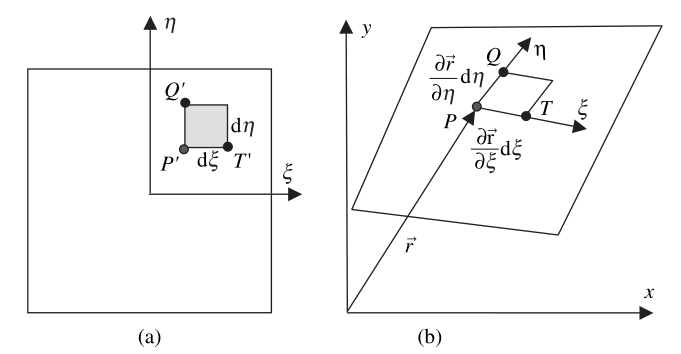
Mapping from the parent(a) to the physical(b) coodrinates system

\(\vec{r}=x\vec{i}+y\vec{j}\)

The vectors \(\vec{a}=\vec{PT}\) and \(\vec{b}=\vec{PQ}\) can be expressed as

\(\vec{a}=\frac{\partial \vec{r}}{\partial \xi}d\xi=(\frac{\partial x}{d\xi}\vec{i}+\frac{\partial y}{d\xi}\vec{j})d\xi\)

\(\vec{b}=\frac{\partial \vec{r}}{\partial \eta}d\eta=(\frac{\partial x}{d\eta}\vec{i}+\frac{\partial y}{d\eta}\vec{j})d\eta\)

$d\Omega=\vec{k}\cdot(\vec{a}\times\vec{b})=\vec{k}\cdot \begin{bmatrix} \vec{i} & \vec{j} & \vec{k}\ \frac{\partial x}{d\xi}d\xi & \frac{\partial y}{d\xi}d\xi & 0\ \frac{\partial x}{d\eta}d\eta & \frac{\partial x}{d\eta}d\eta & 0 \end{bmatrix}= det(\begin{bmatrix} \frac{\partial x}{d\xi} & \frac{\partial y}{d\xi}\ \frac{\partial x}{d\eta} & \frac{\partial x}{d\eta} \end{bmatrix})d\xi d\eta= \vert \pmb{J}^e \vert d\xi d\eta $

\(I=\int\limits_{\eta=-1}^1\int\limits_{\xi=-1}^1\vert \pmb{J}^e(\xi,\eta)\vert f(\xi,\eta) d\xi d\eta=\sum\limits_{i=1}^{n_{gp}}\sum\limits_{j=1}^{n_{gp}}W_iW_j\vert \pmb{J}^e(\xi_i,\eta_j)\vert f(\xi_i,\eta_j)\)

Similar equation can be concluded for three dimensional elements

\(I=\sum\limits_{i=1}^{n_{gp}}\sum\limits_{j=1}^{n_{gp}}\sum\limits_{k=1}^{n_{gp}}W_iW_jW_k\vert \pmb{J}^e(\xi_i,\eta_j,\zeta_k)\vert f(\xi_i,\eta_j,\zeta_k)\)

Integration over triangular elements

\(I=\int\limits_{\Omega}f(\xi,\eta)d\Omega=\sum\limits_{i=1}^{n_{gp}}W_i\vert \pmb{J}^e(\xi_i)\vert f(\xi_i)\)

....